Then and now.
Microstructures evolve. So do the people studying them.

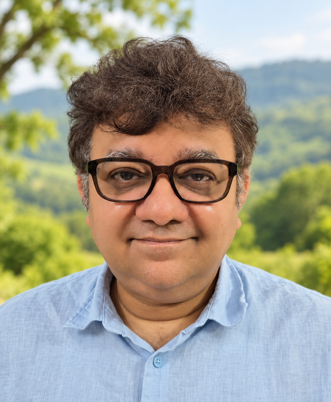
Two photographs, and plenty of learning, questions and confusions in between.
Here I will share my understanding of science, my confusions, questions and things that make me curious. Alongside photographs and observations, I hope this becomes a place to exchange ideas and learn through discussion.
Microstructures evolve. So do the people studying them.
Two photographs, and plenty of learning, questions and confusions in between.
During my Master’s, I saw an animation on the homepage of Prof. W. Craig Carter of MIT. What caught my imagination was not a deep theoretical argument, but an image evolving through an equation. I was really inspired. Sometimes these small encounters become powerful motivating events.
In that spirit, here is my face evolving under two different equations. Inspired by Prof. W. Craig Carter, MIT. His historical homepage shows image evolution under Cahn–Hilliard and Allen–Cahn dynamics.
My portrait is first broken up by shuffling its pixels, producing a distorted, noise-like image. Now define an energy whose minimum is the intact portrait. Both equations move downhill in that energy, and the face emerges as the end product of forward evolution.
Left: Allen–Cahn (nonconserved), \(L=0.03\). Right: Cahn–Hilliard (conserved), \(M=10^{-5}\). Values are dimensionless.
The apparent noise is my color portrait broken up into shuffled pixels. I shuffle whole RGB pixels, so their original colors remain together. As the fields evolve toward the energy minimum, the face returns. The preview shows the final computed frame; press Play to start from the shuffled image.
Build the color example step by step →
I represent the red, green and blue channels by three independent fields. Let \(r_j(x,y)\) be a channel of my fixed portrait and \(u_j(x,y,t)\) the corresponding evolving field. The index \(j\) identifies red, green or blue; \(x,y\) are position coordinates and \(t\) is time. I map each channel's 0–255 values to −1–1. All quantities in this example are dimensionless.
Here \(F\) is the total image energy, \(\Omega\) is the image domain, \(dA\) is an area element, and \(\mu_j\) is the energy derivative for channel \(j\). Every squared difference is nonnegative. The unique unconstrained minimum occurs when every channel matches the portrait: \(\mathbf u=\mathbf r\), where \(F=0\). The symbol on the right is the number zero. This deliberately designed image energy is different from the usual double-well free energy of a material.
\(L=0.03\) sets the Allen–Cahn relaxation rate; \(M=10^{-5}\) is the Cahn–Hilliard mobility. The Laplacian \(\nabla^2\) adds the second spatial derivatives in \(x\) and \(y\). With this local quadratic energy, the Cahn–Hilliard conservation law gives a second-order equation. The familiar fourth-order term would require a gradient-energy contribution, which this restoration example does not include.
With periodic boundaries, both energies decrease:
Cahn–Hilliard preserves the mean of each channel for any initial field. Allen–Cahn does not impose that conservation law. Its channel means approach the target means. Here shuffling preserves all three target means, so the Allen–Cahn means stay fixed as a special case. That does not make Allen–Cahn conserved.
If a starting channel mean differed from its target mean, Cahn–Hilliard would approach the target channel plus a constant offset. The offset equals the initial mean minus the target mean. Allen–Cahn would remove that offset.
I solve the linear equations with exact propagators on a 256 × 256 periodic grid of width 32. The random seed is 19. Frames use nonuniform simulation times, so playback does not compare physical rates. The final frame is calculated at time 30,000,000, rather than replaced by the portrait. The displayed energy is \(F/(3|\Omega|)\), the total energy divided by the domain area \(|\Omega|\) and three channels. Both solutions approach the target asymptotically; a computed zero can occur at finite floating-point precision. Small computed values are shown in scientific notation. Numerical fields are not clipped; clipping is used only to display RGB values.
Download the Python notebook ↓ · Read the code in steps → · Color energy and mean diagnostics ↓ · Download the color animation ↓ · Original grayscale animation ↓
I develop this example in small notebook cells: read the color channels, shuffle whole pixels, check their means, choose the energy, test one evolution step, and then save the full sequence. Each part includes an explanation and a check. Follow the code and its results → · Run the notebook in Colab ↗. The final cells write 241 PNG frames and diagnostics.csv.
Mean drift and motion of the image are different questions. For this energy, the exact Allen–Cahn solution is
Each pixel relaxes toward its fixed target value. This can look like a gradual reveal of the face, but it does not translate the face across the image. A translated portrait is not an energy minimum because the target is tied to fixed positions.
The channel mean obeys the same relaxation rule: \(\overline u_j(t)-\overline r_j=[\overline u_j(0)-\overline r_j]e^{-Lt}\), where the overbar denotes a spatial mean. Thus Allen–Cahn can change the mean when the initial mean differs from the target mean. The shuffled starting image has no such difference.
Other Allen–Cahn models can move interfaces when their free energy supplies a driving force. Motion is possible in those models; the fixed-target energy used here does not demonstrate it.
Here both panels use conserved Cahn–Hilliard dynamics and start from exactly the same portrait with a small, zero-mean perturbation. The left energy favors my portrait. The right energy favors phase separation: my face breaks apart into evolving domains of color, a fun take on abstract art.
The energy determines the destination. The same conserved dynamics can restore a portrait or form color domains, depending on the free-energy functional.
The number shown under each panel is its dimensionless mean energy density: that panel’s total energy \(F\), divided by the image area and by the three RGB channels. It is not an interfacial energy in J m\(^{-2}\). Since the panels use different energy functionals, compare how each number decreases in time, not its magnitude against the other panel.
Allen–Cahn and Cahn–Hilliard are also used in image-processing methods. Edge detection locates boundaries where image brightness or color changes. Image segmentation separates pixels into meaningful regions, such as a particle and the surrounding matrix in a micrograph. Phase-field methods can describe these regions and evolve their boundaries.
For example, Qiao and Zhang combine an edge detector with Allen–Cahn evolution for image segmentation ↗. The detected edges guide the initial field. In another application, Lipková and coauthors use Cahn–Hilliard phase separation to reduce noise and distinguish lesions from healthy tissue in CT images ↗. The image information and the chosen model determine which regions are identified. The portrait animations above illustrate energy-driven evolution; they do not themselves detect edges or identify objects.
I include image-processing applications in the student projects for my Mesoscale Microstructure Modeling course. This is another reason to learn these equations: the same phase-field ideas connect microstructural evolution with the analysis of images. Open the course materials ↗ (access follows the course folder’s permissions).
We treat the red, green and blue channels as three independent signed fields. This is an image analogy, not a coupled material or perceptual color model.
On the right, the portrait supplies the initial field, which evolves under a double-well and gradient energy. On the left, the portrait is explicitly encoded as the energy minimum. Both runs preserve each channel’s mean on the periodic domain. The same zero-mean noise is added to each starting portrait, so the left-hand target is compatible with conservation.
Grid: 256 × 312, spacing 1, M = 1, κ = 0.4. The right-hand nonlinear evolution uses a stabilized semi-implicit Fourier step with Δt = 0.1 and stabilization 2; the left uses the exact linear Fourier propagator. The displayed quantity is \(F/(3|\Omega|)\), a dimensionless mean energy density. The two values belong to different functionals, so their absolute magnitudes should not be compared. Numerical values are not clipped; only displayed RGB values are clipped to the screen’s range. Conservation is checked on the numerical fields.
Learn and run it step by step in Colab ↗ · Download the teaching notebook ↓ · Energy and conservation diagnostics ↓
For discussion: Which image, animation or simple demonstration first made you want to understand the science behind it?
Compare connected regions, periodic wrapping and phase fractions in simulated microstructures. Explore the 2D turtle, the saved 256³ simulation and the topology playground.
Explore connectivity →My wife, Joyita, is an experimentalist who loves to experiment and explore. Having worked on thermoelectrics, she began exploring a thermoelectrics database out of curiosity, using machine learning and SHAP to understand the patterns it contained. She was also looking for patterns in microstructures.
While I was focused on phase-field modeling, she would show me what she was finding. I found the results very informative and began paying closer attention to what AI and machine learning could help us understand. Her curiosity and experiments sparked my own interest. She is the inspiration behind my journey into AI/ML, and I owe this learning to her.
She shares her own explorations, tutorials and examples on Materials Data Explorer ↗.
Some ideas feel clear; others leave me with more questions. This is a space for both, and for the conversations that help us understand them.
The regular-solution model describes a random alloy. Explore why a negative interaction parameter does not by itself describe atomic ordering.
Read the note →Derive the two chemical potentials from a binary molar Gibbs energy curve and explore their tangent intercepts.
Read the note →Compare equal slopes with equal component chemical potentials and see why phase equilibrium requires a common supporting tangent.
Read the note →