My color portrait as an energy minimum

I start with a shuffled color portrait and let it relax toward its original image. I treat red, green and blue as three independent signed fields. The fixed target r is explicitly included in the energy; this is an image analogy, not recovery of an unknown face. Every quantity is dimensionless.

I develop this calculation in small steps. I run a cell, inspect its result and test it before adding the next part. Run the cells in order in Jupyter. A code cell defines a part of the calculation or carries it out; defining a function does not run it.

I permit free noncommercial teaching, learning and demonstrations with acknowledgment. Research and commercial use require my written permission. Earlier licensed releases retain their permissions. Read the code-use terms.

Copyright (c) 2026 Saswata Bhattacharyya.

Step 1: Prepare the Python environment

I install the packages listed in the next cell once in the same environment as the notebook. In Jupyter or Colab, remove the comment marker from the installation line below if a package is missing. NumPy stores arrays and evaluates numerical operations. Matplotlib displays plots. Pillow reads and writes images. This installation does not change the model parameters.

# %pip install numpy "pillow>=10.1" matplotlib
import numpy as np
assert np.isfinite(np.array([0.0, 1.0])).all()
print("NumPy is ready:", np.__version__)

NumPy is ready: 2.1.3

Step 2: Read the image and check its dimensions

I download my public portrait once, or replace this path with my own image. An RGB array has two position axes and one channel axis. The three channels are red, green and blue.

I use Pillow, imported as PIL, to read, resize and save these images. An RGB image with 256 rows and 256 columns has array shape (256, 256, 3). The last 3 counts red, green and blue values at each pixel. It does not represent depth in space. A grayscale image has shape (256, 256) because it has one value per pixel.

target.ndim counts array axes. It is 3 for the RGB array and 2 for the grayscale array. Here a three-axis array still represents a two-dimensional image.

Resizing is different from padding

My source portrait is 1,139 pixels wide and 1,381 pixels high. Its original NumPy RGB shape is (1381, 1139, 3), because NumPy lists rows before columns. Here I resize the complete image to 256 pixels wide and 256 pixels high, giving array shape (256, 256, 3).

There is no padding and no cropping in this operation. Resizing calculates new pixel values from the original image. Because the width and height are changed by different factors, the proportions of the face change too. This simple example uses the specified grid size; it does not preserve the original aspect ratio, meaning width divided by height. To preserve those proportions, we would choose a matching aspect ratio, crop deliberately, or resize proportionally and add explicitly defined borders. Those are different image-preparation choices.

Pillow's resize argument is (width, height). NumPy's image shape is (height, width, channels). These two orders are easy to confuse, so I state both. Resizing also changes the pixel values through interpolation; the resulting target is the resized image, not the full-resolution source portrait.

Adding None to a NumPy index is unrelated to image padding. It adds an array axis of length one without adding a border, changing the spatial grid or introducing new pixel values. The periodic boundary condition used later is also separate: the numerical calculation connects opposite image edges without padding the picture.

from pathlib import Path
from urllib.request import urlretrieve

work = Path("lesson-data")
work.mkdir(exist_ok=True)

def get_file(relative_path):
    # I download a public example only when its local copy is missing.
    destination = work / Path(relative_path).name
    if not destination.exists():
        urlretrieve("https://saswataiith.github.io/" + relative_path, destination)
    return destination

portrait = get_file("assets/images/saswata-landscape.png")
output = "portrait-minimum-results"

Step 3: Import arrays and image operations

I use NumPy for numerical arrays and Pillow for reading images and writing labeled frames. Path handles file locations. The script also imports argparse for its command-line interface; the notebook does not use that interface.

from pathlib import Path
import argparse
import numpy as np
from PIL import Image, ImageDraw, ImageFont

Step 4: A portable display font

I try the original font, then DejaVu Sans, then Pillow's default font. The font changes labels on the image only; it does not change a numerical field.

def portrait_font(size):
    fonts = [Path('/') / 'System' / 'Library' / 'Fonts' / 'Helvetica.ttc', 'DejaVuSans.ttf']
    for font in fonts:
        try:
            return ImageFont.truetype(str(font), size)
        except OSError:
            pass
    return ImageFont.load_default(size=size)

Step 5: Read and shuffle the color pixels

I call the fixed portrait target and the shuffled portrait initial. Each signed RGB channel ranges from −1 to 1. I shuffle whole pixels with seed 19, preserving the three channel means.

def prepare_portrait(path, color=False):
    mode = 'RGB' if color else 'L'
    image = Image.open(path).convert(mode).resize((256, 256))
    target = np.asarray(image, dtype=float) / 127.5 - 1
    rng = np.random.default_rng(19)
    if color:
        initial = rng.permutation(target.reshape(-1, 3), axis=0).reshape(target.shape)
    else:
        initial = rng.permutation(target.ravel()).reshape(target.shape)
    return (target, initial)

Step 6: The discretized evolution equations

I first write the equations that the code evaluates. The fixed target is \(r\) and the evolving image is \(u\). Their difference is \(e=u-r\). I apply the same calculation independently to the red, green and blue channels. All quantities here are dimensionless.

The image grid

There are \(N=256\) grid points along each direction. The periodic domain has width \(\ell=32\), so the grid spacing is \(\Delta x=\Delta y=\ell/N=0.125\). The pixel indices are \(a,b=0,\ldots,N-1\), with positions \(x_a=a\Delta x\) and \(y_b=b\Delta y\). Index \(j\) denotes a color channel. At time \(t_n\), the error at a pixel is \(e^n_{abj}=u^n_{abj}-r_{abj}\).

The discrete energy is

\[F_h=\frac{\Delta x\Delta y}{2}\sum_{a,b,j}(u_{abj}-r_{abj})^2.\]

Here \(F_h\) is the grid approximation of the total energy. Its minimum is zero when every pixel matches the target.

Allen–Cahn: a local update at every pixel

The equation at each grid point is

\[\frac{d e_{abj}}{dt}=-L e_{abj},\qquad L=0.03.\]

Over a time interval \(\Delta t=t_{n+1}-t_n\), its exact update is

\[u^{n+1}_{abj}=r_{abj}+(u^n_{abj}-r_{abj})\exp(-L\Delta t).\]

Every pixel relaxes toward its own target value. Neighboring pixels do not enter this particular Allen–Cahn equation because I have not included a gradient-energy term.

Cahn–Hilliard: an update for each Fourier mode

The error satisfies \(\partial_t e=M\nabla^2e\), with mobility \(M=10^{-5}\). I approximate the spatial derivatives using a discrete Fourier transform on the periodic grid. A hat denotes a Fourier coefficient. The integer mode indices \(p,q\) use NumPy's ordering \(0,1,\ldots,127,-128,\ldots,-1\). Their wave numbers are \(k_p=2\pi p/\ell\) and \(k_q=2\pi q/\ell\).

For a Fourier mode, the Laplacian becomes multiplication by \(-(k_p^2+k_q^2)\):

\[\frac{d\widehat e_{pqj}}{dt}=-M(k_p^2+k_q^2)\widehat e_{pqj}.\]

The exact update for that mode is

\[\widehat e^{n+1}_{pqj}=\widehat e^n_{pqj}\exp[-M(k_p^2+k_q^2)\Delta t].\]

I take the inverse discrete Fourier transform, abbreviated IFFT, to return to pixel values:

\[u^{n+1}_{abj}=r_{abj}+\operatorname{IFFT}_{pq\to ab}(\widehat e^{n+1}_{pqj}).\]

The mode \(p=q=0\) represents the spatial mean. Its multiplying factor is exactly one, so Cahn–Hilliard preserves the mean of each channel. The other modes decay. These are Fourier spatial derivatives, not a nearest-neighbor finite-difference approximation.

Translate these equations into code

The function below evaluates the field directly at the requested time, measured from the initial field at time zero. Therefore its exponent uses time, rather than repeatedly advancing by a chosen time step. This is exact time integration of the spatially discretized linear equations. It is not a forward Euler update.

I keep the grid, rates and numerical calculation unchanged. I name each intermediate quantity so that each line can be compared with the equations above.

Why is there a channel axis in the multiplier?

The squared wave numbers initially form a (256, 256) array, with one value at each pair of spatial Fourier modes. RGB Fourier coefficients have shape (256, 256, 3). I therefore write wave_number_squared[:, :, None] to give the multiplier shape (256, 256, 1). The two colons keep all rows and columns; None adds a last axis of length one. NumPy repeats this same multiplier across the three channels during multiplication. This rule is called broadcasting. There is no Fourier transform along the channel axis.

The if statement checks whether a channel axis is present. It lets the same function handle either an RGB image or a grayscale image. In this color lesson the condition is true.

def evolve(target, initial, time):
    # I keep the original grid and the two relaxation rates.
    grid_points = 256
    domain_width = 32.0
    grid_spacing = domain_width / grid_points
    allen_cahn_rate = 0.03
    cahn_hilliard_mobility = 1e-05

    # I construct the wave numbers for the two position directions.
    wave_numbers = 2 * np.pi * np.fft.fftfreq(grid_points, d=grid_spacing)
    wave_x = wave_numbers[:, None]
    wave_y = wave_numbers[None, :]
    wave_number_squared = wave_x**2 + wave_y**2

    # I check for rows, columns and a color-channel axis.
    # For RGB, I change (256, 256) to (256, 256, 1).
    # NumPy then applies the multiplier to all three channels.
    if target.ndim == 3:
        wave_number_squared = wave_number_squared[:, :, None]

    # I measure the starting difference from the fixed portrait.
    initial_error = initial - target

    # I evaluate the Allen–Cahn error at every pixel.
    ac_decay = np.exp(-allen_cahn_rate * time)
    ac_error = initial_error * ac_decay
    ac = target + ac_error

    # I transform only the position axes, keeping channels separate.
    initial_error_hat = np.fft.fft2(initial_error, axes=(0, 1))
    ch_decay = np.exp(-cahn_hilliard_mobility * wave_number_squared * time)
    ch_error_hat = initial_error_hat * ch_decay
    ch_error = np.fft.ifft2(ch_error_hat, axes=(0, 1)).real
    ch = target + ch_error

    return ac, ch

Step 7: My check of the pixel shuffle

I prepare the target r and starting field u0 as 256 × 256 × 3 arrays. I check that each channel has the same mean before and after shuffling. I display the two arrays side by side; signed values are mapped back to display colors only.

target, initial = prepare_portrait(portrait, color=True)
assert target.shape == initial.shape == (256, 256, 3)
assert np.allclose(initial.mean((0, 1)), target.mean((0, 1)), atol=1e-13, rtol=0)
import matplotlib.pyplot as plt
fig, axes = plt.subplots(1, 2, figsize=(9, 4))
for ax, field, title in zip(axes, (initial, target), ("Shuffled pixels", "Fixed target")):
    ax.imshow(np.clip((field + 1) / 2, 0, 1))
    ax.set_title(title)
    ax.axis("off")
plt.show()
print("Channel means:", initial.mean((0, 1)))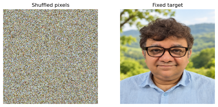

Channel means: [0.25635938 0.23498763 0.09989325]

Step 8: Define energy and verify its minimum

I choose \(F=\tfrac12\int_\Omega\sum_j(u_j-r_j)^2\,dA\). Here \(j\) identifies an RGB channel, \(\Omega\) is the image domain and \(dA\) is an area element. The mean energy density below is \(F/(3|\Omega|)\). Every squared difference is nonnegative, so the minimum is exactly \(F=0\) when \(u=r\). This is the number zero. A finite-time solution approaches this minimum asymptotically.

def mean_energy(field):
    return 0.5 * np.mean((field - target)**2)
assert mean_energy(target) == 0.0
assert mean_energy(initial) > 0.0
print("Target energy:", mean_energy(target))
print("Initial energy:", mean_energy(initial))

Target energy: 0.0
Initial energy: 0.2203078196211593

Step 9: Evaluate at one time and compare the two laws

For channel \(j\), Allen–Cahn gives \(\partial_tu_j=-L(u_j-r_j)\), with \(L=0.03\). Cahn–Hilliard gives \(\partial_tu_j=M\nabla^2(u_j-r_j)\), with \(M=10^{-5}\). Here \(t\) is dimensionless time and \(\nabla^2\) is the spatial Laplacian. This local quadratic energy gives a second-order conserved equation; a gradient energy would supply the familiar fourth-order term. I use the exact propagators at time 100.

ac, ch = evolve(target, initial, 100.0)
assert mean_energy(ac) <= mean_energy(initial)
assert mean_energy(ch) <= mean_energy(initial)
assert np.allclose(ch.mean((0, 1)), initial.mean((0, 1)), atol=2e-13, rtol=0)
fig, axes = plt.subplots(1, 2, figsize=(9, 4))
for ax, field, title in zip(axes, (ac, ch), ("Allen–Cahn, t=100", "Cahn–Hilliard, t=100")):
    ax.imshow(np.clip((field + 1) / 2, 0, 1))
    ax.set_title(title)
    ax.axis("off")
plt.show()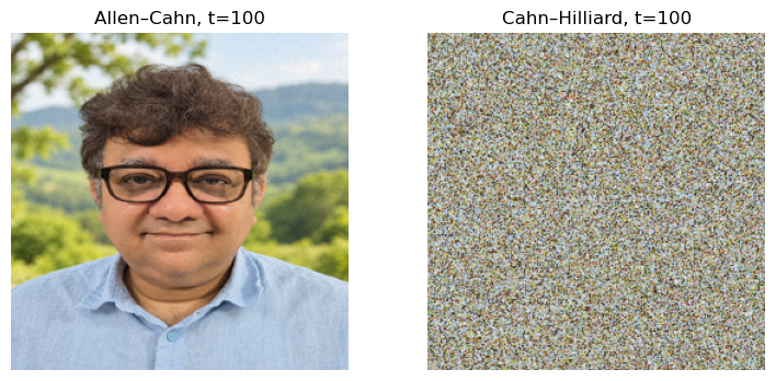

Step 10: Mean drift and spatial motion

I add a spatially uniform offset of 0.1 to the target. Allen–Cahn removes this mean offset exponentially. Cahn–Hilliard preserves it. Neither rule translates the fixed target across the image. Other Allen–Cahn energies can drive interface motion; this example does not test that.

offset_ac, offset_ch = evolve(target, target + 0.1, 100.0)
assert np.allclose(offset_ac - target, 0.1 * np.exp(-0.03 * 100), atol=1e-14)
assert np.allclose(offset_ch - target, 0.1, atol=1e-14)
print("AC remaining offset:", (offset_ac - target).mean())
print("CH remaining offset:", (offset_ch - target).mean())

AC remaining offset: 0.004978706836786389
CH remaining offset: 0.10000000000000003

Step 11: Save the complete portrait sequence

I keep the original grid, seed, time samples and exact propagators. Each saved row contains time, channel means and energy density. The output folder contains 241 image frames and diagnostics.csv. The movie uses nonuniform simulation times, so its playback speed is not a physical rate comparison.

def run_example(portrait, output, color=False):
    output = Path(output)
    output.mkdir(parents=True, exist_ok=True)
    target, initial = prepare_portrait(portrait, color)
    font, small = (portrait_font(25), portrait_font(22))
    records = []
    times = np.r_[0, np.geomspace(0.1, 30000000.0, 240)]
    for index, time in enumerate(times):
        ac, ch = evolve(target, initial, time)
        energies = [0.5 * np.mean((field - target) ** 2) for field in [ac, ch]]
        if color:
            means = [*ac.mean(axis=(0, 1)), *ch.mean(axis=(0, 1))]
        else:
            means = [ac.mean(), ch.mean()]
        records.append([time, *means, *energies])
        frame = Image.new('RGB', (1160, 754), '#f5f7f2')
        draw = ImageDraw.Draw(frame)
        draw.text((24, 14), 'MY PORTRAIT IS THE ENERGY MINIMUM', font=font, fill='#173d40')
        draw.text((24, 51), f'Forward relaxation | time {time:.3g} | L=0.03, M=0.00001 | nonuniform time sampling', font=small, fill='#173d40')
        for x, field, title, energy in [(24, ac, 'Allen-Cahn | nonconserved', energies[0]), (604, ch, 'Cahn-Hilliard | conserved', energies[1])]:
            draw.text((x, 99), title, font=small, fill='#173d40')
            pixels = np.uint8(np.clip((field + 1) * 127.5, 0, 255))
            frame.paste(Image.fromarray(pixels).resize((528, 528)), (x, 139))
            if color:
                draw.text((x, 687), f'F / (3 x area): {energy:.3e}', font=small, fill='#173d40')
                rgb = field.mean(axis=(0, 1))
                draw.text((x, 718), 'Mean R/G/B: ' + ' / '.join((f'{v:+.3f}' for v in rgb)), font=small, fill='#173d40')
            else:
                draw.text((x, 687), f'Energy / area: {energy:.7f}', font=small, fill='#173d40')
                draw.text((x, 718), f'Mean field: {field.mean():+.5f}', font=small, fill='#173d40')
        frame.save(output / f'frame-{index:03d}.png')
    initial_mean = initial.mean(axis=(0, 1))
    assert np.max(np.abs(ch.mean(axis=(0, 1)) - initial_mean)) < 1e-10
    assert max(energies) < 1e-06
    if color:
        header = 'time,AC_R_mean,AC_G_mean,AC_B_mean,CH_R_mean,CH_G_mean,CH_B_mean,AC_energy_per_area_per_channel,CH_energy_per_area_per_channel'
    else:
        header = 'time,AC_mean,CH_mean,AC_energy_per_area,CH_energy_per_area'
    np.savetxt(output / 'diagnostics.csv', records, delimiter=',', header=header, comments='')
    print('Final energy densities:', energies)
    print('CH maximum channel mean drift:', np.max(np.abs(ch.mean(axis=(0, 1)) - initial_mean)))

Step 12: Save the original 241-frame color calculation

I now use the complete frame writer defined in the preceding cell. I preserve the original nonuniform sample times, ending at 30,000,000. The PNG files and diagnostics.csv are written in the chosen output folder. Frames are not uniformly spaced in simulation time.

run_example(portrait, output, color=True)

Final energy densities: [np.float64(0.0), np.float64(3.8152048054083335e-12)]
CH maximum channel mean drift: 1.2245759961615477e-13

Step 13: Plot energy and check every saved mean

I read the measured diagnostics, rather than infer conservation from the colors. Both energy sequences must be nonincreasing within the stated round-off tolerance. Each Cahn–Hilliard channel mean must remain within 2×10⁻¹³ of its initial value.

records = np.loadtxt(Path(output) / "diagnostics.csv", delimiter=",", skiprows=1)
assert records.shape == (241, 9)
assert np.isfinite(records).all()
assert np.max(np.abs(records[:, 4:7] - records[0, 4:7])) < 2e-13
assert np.max(np.diff(records[:, 7:9], axis=0)) < 1e-15
plt.figure(figsize=(7, 4))
for col, name in [(7, "Allen–Cahn"), (8, "Cahn–Hilliard")]:
    positive = records[:, col] > 0
    plt.loglog(records[positive, 0], records[positive, col], label=name)
plt.xlabel("Dimensionless time")
plt.ylabel("Mean energy density F / (3 × area)")
plt.legend()
plt.show()
print("Final mean energy densities:", records[-1, 7:9])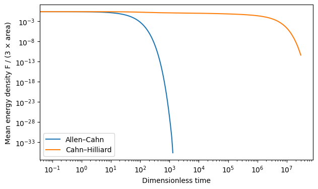

Final mean energy densities: [0.00000000e+00 3.81520481e-12]

Step 14: Review and extend the calculation

I first restart the kernel and run all the required cells. Then I change one input, predict its effect and compare the result with that prediction. A successful check establishes the tested property; it does not establish convergence or equilibrium. I retain the complete script for command-line use. The notebook embeds the calculation directly and does not need that script to run.

Read the notebook execution checks → · More Python, Julia and C lessons →