It looks like a labyrinth.
Is it really bicontinuous?
Books often describe spinodal microstructures as “bicontinuous.” At an average composition of 0.5, the picture may look convincing. But at 0.4, where is the bicontinuity? And even at 0.5, what exactly have we established by looking at a two-dimensional image?
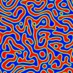
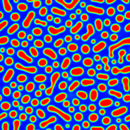
These are computed teaching microstructures, not experimental photographs: 256 × 256 periodic grids, the same initial perturbation (seed 20260921), dimensionless time 400, Δt = 0.2, Δx = 1, and no elastic contribution. Fixed rainbow scale: c = 0 blue, 0.5 green, 1 red. The chemical free-energy density is \(f(c)=A c^2(1-c)^2\), with \(A=1\) and \(M=\kappa=1\). Its bulk coexistence compositions are 0 and 1.
First, what do we mean by “continuous”?
A useful operational definition is that each phase contains a connected network extending across the material over the directions and length scales of interest. Some definitions demand that each entire phase be connected; others allow isolated pockets provided each phase has a spanning network. We should state which meaning we use. A winding stripe, a branching network, and disconnected curved islands are different structures even when all look labyrinthine.
Explore the spinodal labyrinth at mean c = 0.5.
Let the classic KTurtle explore this computed microstructure. Its center stays inside the chosen phase. Click a point to ask: can I get there without crossing the other phase? The black-and-white dash-dot line follows the middle of the channel; the turtle follows this route. Destinations move to a nearby channel center. If a destination is unreachable, watch the turtle try seven blocked moves before asking “Help me!” You can also try a trapped region below.
Loading the spinodal field…
The route uses the same c = 0.5 simulation shown above, split at c = 0.5 with four edge-sharing neighbors. The turtle is enlarged so we can see it; its center marks the tested pixel. Reaching a destination proves a path between two points, not bicontinuity of both phases. Try each phase and compare with the connectivity measurements below. Crossing an edge alone does not prove a wrapping loop.
Turtle artwork: KDE KTurtle, GPL version 2 or later.
Why can the red turtle become trapped?
Periodicity identifies opposite boundaries: leaving one edge returns to the corresponding point on the other. Connectivity still requires every step, including a boundary step, to stay in the selected phase. Periodicity does not join disconnected islands. In this saved 2D field, the red phase has 16 components and no periodic wrapping loop; the largest blue component wraps in both directions. Four edge-sharing neighbors are used. Allowing diagonal contacts does not restore red wrapping.
Mean composition c̄ = 0.5 is a global conservation condition. Threshold c = 0.5 is the separate rule assigning pixels to red or blue. Equal mean composition guarantees neither equal connectedness nor exactly equal thresholded areas: here red occupies about 49.86%.
The symmetric free energy f(c) = f(1−c) makes a solution and its phase-swapped counterpart equally admissible. This symmetry belongs to the equations and statistical ensemble; the two phases need not have identical topology in each finite realization.
Two disjoint networks cannot cross in a plane. Both phases can nevertheless form parallel spanning bands, so bicontinuity is possible in 2D. Three dimensions permit much richer interpenetrating networks. The example below demonstrates measured bicontinuity in one specific simulated 3D field.
These connectivity calculations establish the topology of the saved discrete fields. They do not establish numerical convergence or show that either topology is representative of symmetric spinodal decomposition. Grid refinement, timestep reduction, multiple seeds and different coarsening times are needed to investigate robustness; those studies have not been completed here.
Topology and connectivity: tutorial, experiments and worked solutions →
Flood each phase from one seed.
The original 3D spinodal simulation remains available: Download the Python notebook ↓ · Read the code in steps → and its saved 256³ composition field. The playground explores that fixed simulation output.
In the saved 256 × 256 × 256 microstructure, one seed reaches every red voxel; a second seed reaches every blue voxel. Watch a bright front advance through three movable sections, rotate the linked Plotly view, switch phases, and see both connected clusters fill completely. An editable pattern lab animates how cluster labels merge. The flood explores the whole periodic 3D volume, so regions that look isolated in one section can connect outside that plane.
Open the connectivity explorer →
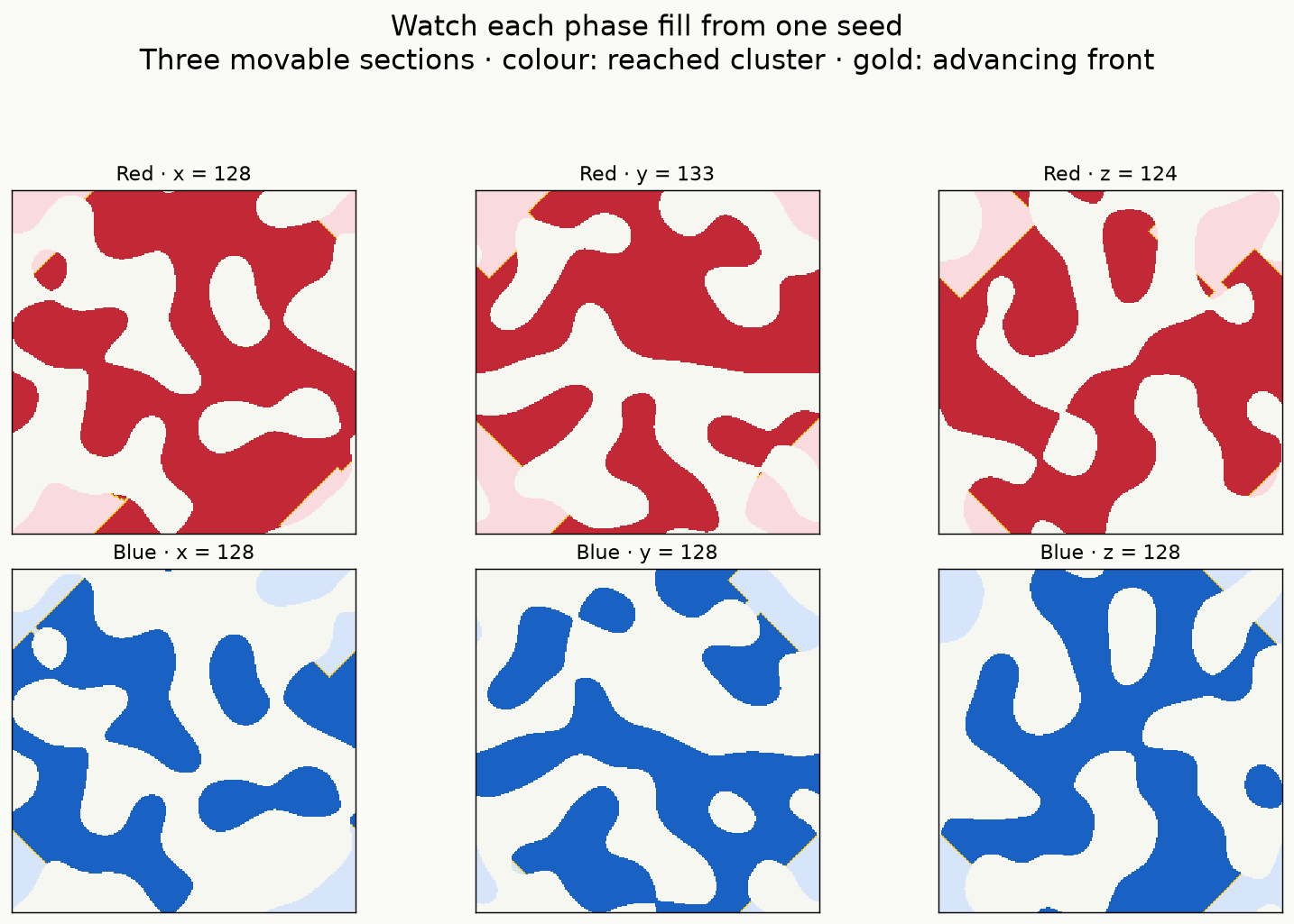
Hoshen–Kopelman style label-and-merge analysis independently confirms one component and winding rank three for both phases at thresholds 0.45, 0.50 and 0.55. Periodic interface area, curvature and Euler characteristic are measured on the unsimplified mesh. Downloads include reproducible source and exact flood distances. The simulation remains fixed; this animation shows graph exploration.
Two dimensions are not three dimensions.
Why demonstrate this in 3D? To demonstrate two interpenetrating phase networks throughout a three-dimensional material, we must inspect the 3D field and measure connectivity in both phases. A labyrinthine 2D image alone is insufficient. In 2D, both phases can span as non-crossing bands, including curved or wavy bands: exact parallelism is not required. During coarsening, pinching off or reconnecting a band can break one phase’s spanning connection. In 3D, paths can pass around one another, allowing much richer interpenetrating networks. Even then, bicontinuity must be checked rather than assumed.
In a plane, one path cannot pass over another without crossing it. Two phases can both extend along parallel stripes, but that does not establish a connected network in every direction. A 2D slice can also cut a connected 3D phase into apparently separate islands. Conversely, a genuinely 2D simulation should not be interpreted as evidence for a 3D interconnected structure.
Periodic boundaries matter too: opposite edges of these images are identified. Connectivity must be assessed on that periodic domain. Touching an image edge is not by itself proof that a phase wraps around the domain.
Measure it instead of naming it from appearance.
For this pair, we split the diffuse composition field at a threshold and count connected components using edge-sharing pixels (four-neighbor connectivity). We also track noncontractible loops: a component “wraps x” or “wraps y” when it contains a path around the periodic domain in that direction. A connection only at a pixel corner is excluded. This is a stated digital convention, not a threshold-independent verdict about continuum morphology.
Composition and phase fraction: the lever rule.
For bulk phases at \(c_0=0\) and \(c_1=1\), the lever rule gives
Thus the ideal phase fractions are 50% high-c / 50% low-c at mean composition 0.5, and 40% high-c / 60% low-c at mean composition 0.4. Here composition is scaled between the two bulk minima, and fractions refer to area in this two-dimensional model.
The ideal bulk phase fraction below follows this lever rule exactly. The measured region area counts pixels above or below the selected threshold in the actual diffuse field. At finite time, interfaces and departures from the bulk endpoint compositions make those two quantities differ. Changing the threshold changes the geometric measurement, not the conserved mean or the ideal lever-rule fractions. “Largest component” is expressed as a percentage of the measured region area.
| Mean composition | Measured region | Ideal bulk phase fraction | Measured region area | Connected components | Largest component (% of region) | Periodic wrapping |
|---|
Do we need differential geometry and topology?
Topology answers the connectivity question: components, loops, holes, and percolating paths. Differential geometry describes the shape of an interface, including its length, area and curvature, and helps explain how it evolves. They complement each other. We do not need a full course in either subject to begin: labeling connected components and testing spanning or periodic wrapping is already much stronger than judging a picture.
Betti numbers count components and independent loops; Euler characteristic combines such information. But a single Euler characteristic does not uniquely specify a network or prove percolation. Its interpretation also depends on boundary conditions.
The discussion I want to have: when we say “bicontinuous,” which phase definition, connectivity rule, boundary condition, direction and observation scale are we assuming? Composition 0.5 does not certify it, and composition 0.4 does not universally rule it out. One simulation, seed and time is an example, not a universal threshold.
Download the Python notebook ↓ · Read the code in steps → · Download measurements ↓
Related research: Two-dimensional bicontinuous structures from symmetric surface-directed spinodal decomposition in thin films; Topology and control of self-assembled domain patterns in low-dimensional ferroelectrics. These illustrate why geometry and connectivity need explicit analysis; they are not validation of this particular teaching calculation.