Structure function
and pair correlation.

Python notebook ↓ · Complete worked Python code ↓

I use NumPy here to present my calculation in small, runnable steps. To analyze a simulated field, first work through the ternary spinodal notebook, then read one composition array from its saved ternary-fields.npz file.

Step 1: A field with known correlation

I choose a cosine composition wave on a periodic 16 by 16 grid. The composition c is dimensionless. Grid spacings dx and dy are one dimensionless length unit. Rows index x and columns index y, following the saved simulation arrays. The wave varies in x and is constant in y, so I can check the full directional result before averaging over directions.

Python

import numpy as np
n = 16
dx = dy = 1.0
x = np.arange(n) * dx
composition = 0.5 + 0.2 * np.cos(2 * np.pi * x[:, None] / (n * dx)) * np.ones((1, n))
assert composition.shape == (n, n)
assert abs(composition.mean() - 0.5) < 1e-12
print("Mean composition:", composition.mean())

Step 2: Remove the mean and calculate the variance

I use the fluctuation δc = c minus the measured mean of this field. Its variance is the mean of δc². Removing the actual mean avoids a residual zero mode when a nominal alloy composition differs from the saved field mean.

Python

fluctuation = composition - composition.mean()
variance = np.mean(fluctuation**2)
assert abs(fluctuation.mean()) < 1e-12
assert abs(variance - 0.02) < 1e-12
print("Composition variance:", variance)

Step 3: Calculate the structure function

I define F as the unnormalized forward discrete Fourier transform of δc and N as the total number of grid cells. The structure function is S = |F|²/N. Its units are squared composition units under this discrete convention; here they are dimensionless. It is nonnegative. Its sum divided by N equals the real-space variance. This check detects normalization errors.

Python

cells = composition.size
transform = np.fft.fft2(fluctuation)
structure = np.abs(transform)**2 / cells
assert np.all(structure >= 0)
assert abs(structure[0, 0]) < 1e-12
assert abs(structure.sum() / cells - variance) < 1e-12
print("Parseval check:", structure.sum() / cells, variance)

Step 4: Invert the spectrum to obtain pair correlation

The unnormalized covariance C at displacement r is the spatial average of δc(x)δc(x+r). With NumPy’s normalized inverse transform, C = ifft2(S).real. I define the normalized correlation ρ = C/C(0). The origin must be one. A constant field has zero variance, so its normalized correlation is undefined; I reject it rather than divide by zero.

Python

def correlation_from_field(field):
    deviation = field - field.mean()
    variance = np.mean(deviation**2)
    if variance == 0:
        raise ValueError("A constant field has undefined normalized correlation.")
    structure = np.abs(np.fft.fft2(deviation))**2 / field.size
    covariance = np.fft.ifft2(structure).real
    return structure, covariance, covariance / variance

structure, covariance, correlation = correlation_from_field(composition)
assert abs(covariance[0, 0] - variance) < 1e-12
assert abs(correlation[0, 0] - 1) < 1e-12
try:
    correlation_from_field(np.ones((4, 4)))
except ValueError:
    print("Constant-field check passed.")
else:
    raise AssertionError("The constant field must be rejected.")

Step 5: My direct-sum check at each displacement

I now calculate the same covariance without using a Fourier transform. np.roll implements periodic displacements. This direct calculation is slow for large grids, but useful as an independent check on a small grid. The cosine field should give ρ(r_x,r_y) = cos(2π r_x/L_x), independent of r_y.

Python

direct = np.zeros_like(composition)
for row in range(n):
    for column in range(n):
        shifted = np.roll(fluctuation, (row, column), axis=(0, 1))
        direct[row, column] = np.mean(fluctuation * shifted)
expected = np.cos(2 * np.pi * np.arange(n)[:, None] / n) * np.ones((1, n))
assert np.max(np.abs(direct - covariance)) < 1e-12
assert np.max(np.abs(correlation - expected)) < 1e-12
print("Direct-sum maximum error:", np.max(np.abs(direct - covariance)))

Step 6: Average by radius only after checking the directional data

For the correlation I bin by real-space displacement radius r, in length units, using minimum-image displacements. For the structure function I bin by wave-number magnitude k, in inverse-length units. They need separate radii and bin widths. Radial averaging discards direction information and can conceal anisotropy. Empty bins are omitted rather than divided by zero.

Python

def radial_average(values, radii, bin_width):
    bins = np.floor(radii / bin_width + 0.5).astype(int)
    occupied_bins = np.unique(bins)
    centers = occupied_bins * bin_width
    means = np.array([values[bins == index].mean() for index in occupied_bins])
    counts = np.array([np.count_nonzero(bins == index) for index in occupied_bins])
    return centers, means, counts

rx = np.fft.fftfreq(n) * n * dx
ry = np.fft.fftfreq(n) * n * dy
real_radius = np.sqrt(rx[:, None]**2 + ry[None, :]**2)
kx = 2 * np.pi * np.fft.fftfreq(n, d=dx)
ky = 2 * np.pi * np.fft.fftfreq(n, d=dy)
wave_radius = np.sqrt(kx[:, None]**2 + ky[None, :]**2)
r, radial_correlation, counts = radial_average(correlation, real_radius, min(dx, dy))
k, radial_structure, mode_counts = radial_average(structure, wave_radius, min(2*np.pi/(n*dx), 2*np.pi/(n*dy)))
assert counts.sum() == cells and mode_counts.sum() == cells
assert radial_correlation[0] == correlation[0, 0]
print("Correlation radii:", r)
print("Wave-number magnitudes:", k)

Step 7: Report a first zero only if one is present

A first zero is one possible characteristic length. I find the first positive-to-nonpositive crossing and linearly interpolate between the sampled values. If no such crossing is present in the sampled range, I return None. This is not automatically a particle radius, and it is not a connectivity measurement. For the directional cosine test, the first zero is at one quarter of the wavelength.

Python

def first_zero(distances, values):
    for index in range(1, len(values)):
        if values[index - 1] > 0 and values[index] <= 0:
            fraction = values[index - 1] / (values[index - 1] - values[index])
            return distances[index - 1] + fraction * (distances[index] - distances[index - 1])
    return None

directional_zero = first_zero(x[:n//2+1], correlation[:n//2+1, 0])
assert abs(directional_zero - n * dx / 4) < 1e-12
assert first_zero(np.arange(3), np.ones(3)) is None
print("Directional first zero:", directional_zero)
print("Radial first zero:", first_zero(r, radial_correlation))

import matplotlib.pyplot as plt
fig, axes = plt.subplots(1, 2, figsize=(9, 4))
axes[0].plot(k, radial_structure, "o-")
axes[0].set_xlabel("Wave-number magnitude k (inverse length units)")
axes[0].set_ylabel("Radial structure function S (dimensionless)")
axes[1].plot(r, radial_correlation, "o-", label="Radial average")
axes[1].plot(x[:n//2+1], correlation[:n//2+1, 0], "--", label="x direction")
axes[1].axhline(0, color="gray", linewidth=0.7)
axes[1].set_xlabel("Displacement radius r (length units)")
axes[1].set_ylabel("Normalized correlation (dimensionless)")
axes[1].legend()
fig.tight_layout()
plt.show()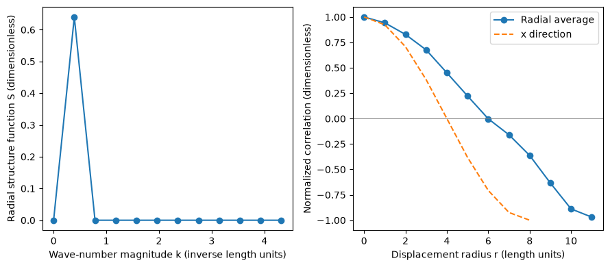

Fourier normalization

FFTW uses an unnormalized backward transform. The original convention S = |F|²/N therefore needs division by N after the backward transform to obtain covariance, followed by division by variance for normalized correlation. NumPy already includes that backward-transform division; applying it again would be an error.

Return to the step-by-step code collection →