Ternary spinodal decomposition.
Build the calculation in steps.

The calculation, one step at a time

I show the purpose of each notebook cell beside its code and recorded result. The controls move through those results; they do not execute Python in the browser. The notebook remains available for running or changing the calculation.

Loading the lesson…

Step 1: Create the grid and initial compositions

I use 256 points in each direction. The grid spacings dx and dy are one dimensionless length unit. The seed fixes the random starting field. I remove the mean of each small fluctuation so the initial mean of each component is exactly one third to numerical precision. These fluctuations are added only at initialization.

Python

import numpy as np
import matplotlib.pyplot as plt

Nx = Ny = 256
dx = dy = 1.0
seed = 1234
rng = np.random.RandomState(seed)
noise_A = rng.normal(0.0, 0.001, (Nx, Ny))
noise_B = rng.normal(0.0, 0.001, (Nx, Ny))
cA = 1.0 / 3.0 + noise_A - noise_A.mean()
cB = 1.0 / 3.0 + noise_B - noise_B.mean()
cC = 1.0 - cA - cB
initial_A, initial_B = cA.copy(), cB.copy()
initial_means = np.array([cA.mean(), cB.mean(), cC.mean()])
assert np.max(np.abs(initial_means - 1.0 / 3.0)) < 1e-12
print("Initial mean mole fractions:", initial_means)

Step 2: The polynomial free energy

I define the bulk free-energy density as \[f=A_1c_A^2c_B^2+A_2c_B^2c_C^2+A_3c_A^2c_C^2+B c_A^2c_B^2c_C^2.\] The coefficients A1, A2, A3 and B are dimensionless free-energy parameters. B is a coefficient, not the mole fraction cB. I use A1 = A2 = A3 = 1 and B = 12 from my notebook. This is a polynomial model, rather than the regular-solution model with logarithms. Its three pure-component corners have zero bulk energy. The total free energy adds kA|∇cA|² + kB|∇cB|² + kC|∇cC|², where kA, kB and kC are dimensionless gradient-energy coefficients.

Python

A1 = A2 = A3 = 1.0
B = 12.0
kA = kB = kC = 1.0
kAA, kBB, kAB = kA + kC, kB + kC, kC

def bulk_energy(a, b):
    c = 1.0 - a - b
    return A1*a**2*b**2 + A2*b**2*c**2 + A3*a**2*c**2 + B*a**2*b**2*c**2

assert bulk_energy(1.0, 0.0) == 0.0
assert bulk_energy(0.0, 1.0) == 0.0
assert bulk_energy(0.0, 0.0) == 0.0
print("Bulk energy at equal composition:", bulk_energy(1/3, 1/3))

Step 3: Differentiate while enforcing the composition constraint

I substitute cC = 1 − cA − cB before differentiating. The derivatives gA = ∂f/∂cA and gB = ∂f/∂cB are diffusion-potential differences relative to C. They are dimensionless here. I compare the analytical expressions with centered finite differences at several compositions before using them in evolution.

Python

def bulk_derivatives(a, b):
    c = 1.0 - a - b
    gA = (2*A1*a*b**2 - 2*A2*b**2*c
          + 2*A3*a*c**2 - 2*A3*a**2*c
          + 2*B*a*b**2*c**2 - 2*B*a**2*b**2*c)
    gB = (2*A1*a**2*b + 2*A2*b*c**2
          - 2*A2*b**2*c - 2*A3*a**2*c
          + 2*B*a**2*b*c**2 - 2*B*a**2*b**2*c)
    return gA, gB

check_points = rng.dirichlet([1, 1, 1], size=100)
a, b = check_points[:, 0], check_points[:, 1]
eps = 1e-6
gA, gB = bulk_derivatives(a, b)
fd_A = (bulk_energy(a+eps, b) - bulk_energy(a-eps, b)) / (2*eps)
fd_B = (bulk_energy(a, b+eps) - bulk_energy(a, b-eps)) / (2*eps)
derivative_error = max(np.max(np.abs(gA-fd_A)), np.max(np.abs(gB-fd_B)))
assert derivative_error < 1e-8
print("Maximum derivative error:", derivative_error)

Step 4: Define mobility and check its sign

I write the constant mobility matrix explicitly: \[L=\begin{pmatrix}M_{AA}&-M_{AB}\\-M_{AB}&M_{BB}\end{pmatrix}. \qquad \partial_t\mathbf c=\nabla\cdot(L\nabla\boldsymbol\mu).\] Here the composition vector is (cA,cB), and the diffusion-potential vector is (μA,μB). I retain the original notation MAB = 0.5 as the positive magnitude; the actual off-diagonal entries are −0.5. The mobility coefficients are dimensionless. Positive eigenvalues ensure that the continuum free-energy rate is nonpositive: dF/dt = −∫(∇μ)ᵀL(∇μ) dA. This does not prove stability of a finite time step.

Python

M_AA = M_BB = 1.0
M_AB = 0.5
mobility = np.array([[M_AA, -M_AB], [-M_AB, M_BB]])
assert np.all(np.linalg.eigvalsh(mobility) > 0)
print("Mobility eigenvalues:", np.linalg.eigvalsh(mobility))

Step 5: Construct the Fourier wave numbers

I use NumPy's frequency order to construct kx and ky, in inverse dimensionless length units. The quantity k2 = kx² + ky² is the squared wave-number magnitude. k4 = k2². A Fourier Laplacian multiplies by −k2. The gradient contribution contains two Laplacians, so it produces k4. The zero mode has k2 = 0 and must remain unchanged.

Python

kx = 2*np.pi*np.fft.fftfreq(Nx, d=dx)
ky = 2*np.pi*np.fft.fftfreq(Ny, d=dy)
k2 = kx[:, None]**2 + ky[None, :]**2
k4 = k2**2
assert k2[0, 0] == 0.0
assert k2.shape == cA.shape
print("Maximum squared wave number:", k2.max())

Step 6: Solve one coupled time step

I define the gradient-coefficient matrix K with entries kAA, kBB and kAB. Because the gradient energy has no factor one half, μ = g − 2K∇²c. I treat g explicitly and the coupled gradient terms implicitly: \[[I+2\Delta t\,k^4 LK]\widehat{\mathbf c}^{\,new} =\widehat{\mathbf c}^{\,old}-\Delta t\,k^2L\widehat{\mathbf g}^{\,old}.\] The hat denotes the discrete Fourier transform, I is the identity matrix, and dt is the dimensionless time step. I write the two-by-two solution explicitly so both new fields use the same old fields. In my original notebook the second assignment used an already updated first field; this teaching version removes that ordering dependence.

Python

dt = 0.1
K = np.array([[kAA, kAB], [kAB, kBB]])
LK = mobility @ K
H11 = 1 + 2*dt*k4*LK[0, 0]
H12 = 2*dt*k4*LK[0, 1]
H21 = 2*dt*k4*LK[1, 0]
H22 = 1 + 2*dt*k4*LK[1, 1]
determinant = H11*H22 - H12*H21
assert np.all(determinant > 0)

def advance(a, b):
    gA, gB = bulk_derivatives(a, b)
    a_hat, b_hat = np.fft.fft2(a), np.fft.fft2(b)
    gA_hat, gB_hat = np.fft.fft2(gA), np.fft.fft2(gB)
    rhs_A = a_hat - dt*k2*(M_AA*gA_hat - M_AB*gB_hat)
    rhs_B = b_hat - dt*k2*(M_BB*gB_hat - M_AB*gA_hat)
    new_A_hat = (H22*rhs_A - H12*rhs_B) / determinant
    new_B_hat = (H11*rhs_B - H21*rhs_A) / determinant
    return np.fft.ifft2(new_A_hat).real, np.fft.ifft2(new_B_hat).real

one_A, one_B = advance(cA, cB)
assert abs(one_A.mean() - cA.mean()) < 1e-12
assert abs(one_B.mean() - cB.mean()) < 1e-12
print("One-step conservation check passed.")

Step 7: Repeat the update and measure conservation

I now run 20000 steps, giving a final dimensionless time of 2000, as in my original notebook. For a quick first check, students can reduce steps to 2000. I record the mean and minimum and maximum mole fractions every 100 steps. The polynomial model does not guarantee that every mole fraction stays between zero and one. I report these values and do not clip the evolving fields, because clipping changes component conservation.

Python

steps = 20000
cA, cB = initial_A.copy(), initial_B.copy()
history = []
for n in range(steps + 1):
    if n % 100 == 0 or n == steps:
        cC = 1.0 - cA - cB
        fields = np.array([cA, cB, cC])
        assert np.all(np.isfinite(fields))
        means = fields.mean(axis=(1, 2))
        drift = np.max(np.abs(means - initial_means))
        history.append([n*dt, drift, fields.min(), fields.max()])
    if n < steps:
        cA, cB = advance(cA, cB)
cC = 1.0 - cA - cB
history = np.array(history)
assert history[:, 1].max() < 1e-11
print("Final time:", steps*dt)
print("Maximum mean drift:", history[:, 1].max())
print("Final minimum and maximum:", min(cA.min(), cB.min(), cC.min()), max(cA.max(), cB.max(), cC.max()))

Step 8: Three composition regions in one microstructure

I use the pastel map from my saved ternary analysis code. At each grid cell, I compare the dimensionless mole fractions cA, cB and cC. The largest fraction determines the color: slate blue for A-rich regions, sage green for B-rich regions and clay for C-rich regions. I shade the color using the difference between the largest and second-largest fractions. Black lines mark where neighboring grid cells change their composition label. I include neighbors across the periodic boundaries. The Gibbs-triangle legend uses the same colors and shading. Its corners are pure A, B and C. These labels help us see the three regions together; they are a display classification, not a separate calculation of thermodynamic phase equilibrium. The black lines are drawn for clarity and do not indicate a fourth phase or the physical width of a diffuse interface. At an exact tie, NumPy selects the first largest fraction; the corresponding boundary is visible in the legend. I retain my continuous color_ps-style RGB map as an alternative. Set display_style = "rgb" to show R = cA, G = cB and B = cC. That view shows intermediate compositions directly. The pastel map has its own color assignments, as shown in its legend. The field has a small negative overshoot. I limit only displayed color values to [0,1]; I do not alter the simulation. The horizontal axis indexes y and the vertical axis indexes x. Nearest-neighbor display adds no extra interpolated colors between grid cells.

Python

def composition_rgb(a, b, c):
    # I retain my continuous RGB map as an alternative view of composition.
    return np.clip(np.stack([a, b, c], axis=-1), 0.0, 1.0)


def composition_pastel(a, b, c, draw_edges=True, periodic=True):
    # I assign one color according to the largest local mole fraction.
    composition = np.clip(np.stack([a, b, c], axis=-1), 0.0, 1.0)
    label = np.argmax(composition, axis=-1)
    palette = np.array([[130, 160, 195], [170, 185, 140], [200, 145, 125]]) / 255.0
    color = palette[label].copy()

    # I use the difference between the largest two fractions to shade each region.
    ordered = np.sort(composition, axis=-1)
    difference = ordered[..., -1] - ordered[..., -2]
    brightness = 0.65 + 0.35 * np.clip(difference / 0.7, 0.0, 1.0)
    color *= brightness[..., None]

    # I draw black lines where neighboring grid cells have different labels.
    if draw_edges:
        edge = np.zeros(label.shape, dtype=bool)
        if periodic:
            for axis in (0, 1):
                edge |= label != np.roll(label, 1, axis=axis)
                edge |= label != np.roll(label, -1, axis=axis)
        else:
            edge[:-1, :] |= label[:-1, :] != label[1:, :]
            edge[1:, :] |= label[1:, :] != label[:-1, :]
            edge[:, :-1] |= label[:, :-1] != label[:, 1:]
            edge[:, 1:] |= label[:, 1:] != label[:, :-1]
        color[edge] = 0.0
    return color


# I can choose "pastel" for clear regions or "rgb" for continuous composition colors.
display_style = "pastel"
before_plot = np.stack([cA, cB, cC]).copy()
if display_style == "pastel":
    image = composition_pastel(cA, cB, cC)
else:
    image = composition_rgb(cA, cB, cC)
assert image.shape == (Nx, Ny, 3)
assert np.array_equal(before_plot, np.stack([cA, cB, cC]))

# I construct a Gibbs-triangle legend with the same colors and shading.
height = np.sqrt(3.0) / 2.0
xx, yy = np.meshgrid(np.linspace(0.0, 1.0, 401), np.linspace(0.0, height, 349))
legend_C = yy / height
legend_B = xx - legend_C / 2.0
legend_A = 1.0 - legend_B - legend_C
inside = (legend_A >= 0) & (legend_B >= 0) & (legend_C >= 0)
if display_style == "pastel":
    legend_color = composition_pastel(legend_A, legend_B, legend_C, periodic=False)
    labels = ("A-rich\nSlate blue", "B-rich\nSage green", "C-rich\nClay")
else:
    legend_color = composition_rgb(legend_A, legend_B, legend_C)
    labels = ("A-rich\nRed", "B-rich\nGreen", "C-rich\nBlue")
legend_rgba = np.dstack([legend_color, inside.astype(float)])

fig, (ax, triangle) = plt.subplots(1, 2, figsize=(11, 5.5),
                                  gridspec_kw={"width_ratios": [1.3, 1]},
                                  constrained_layout=True)
ax.imshow(image, origin="lower", interpolation="nearest")
ax.set_title("Ternary microstructure\nDimensionless time " + str(steps*dt))
ax.set_xlabel("y index (grid cells)")
ax.set_ylabel("x index (grid cells)")
triangle.imshow(legend_rgba, extent=[0, 1, 0, height], origin="lower", interpolation="nearest")
triangle.plot([0, 1, 0.5, 0], [0, 0, height, 0], color="#26333c", lw=1)
triangle.text(0, -0.045, labels[0], ha="center", va="top")
triangle.text(1, -0.045, labels[1], ha="center", va="top")
triangle.text(0.5, height+0.045, labels[2], ha="center", va="bottom")
triangle.set_title("Gibbs-triangle color legend", pad=28)
triangle.set_xlim(-0.12, 1.12)
triangle.set_ylim(-0.14, height+0.14)
triangle.set_aspect("equal")
triangle.axis("off")
plt.show()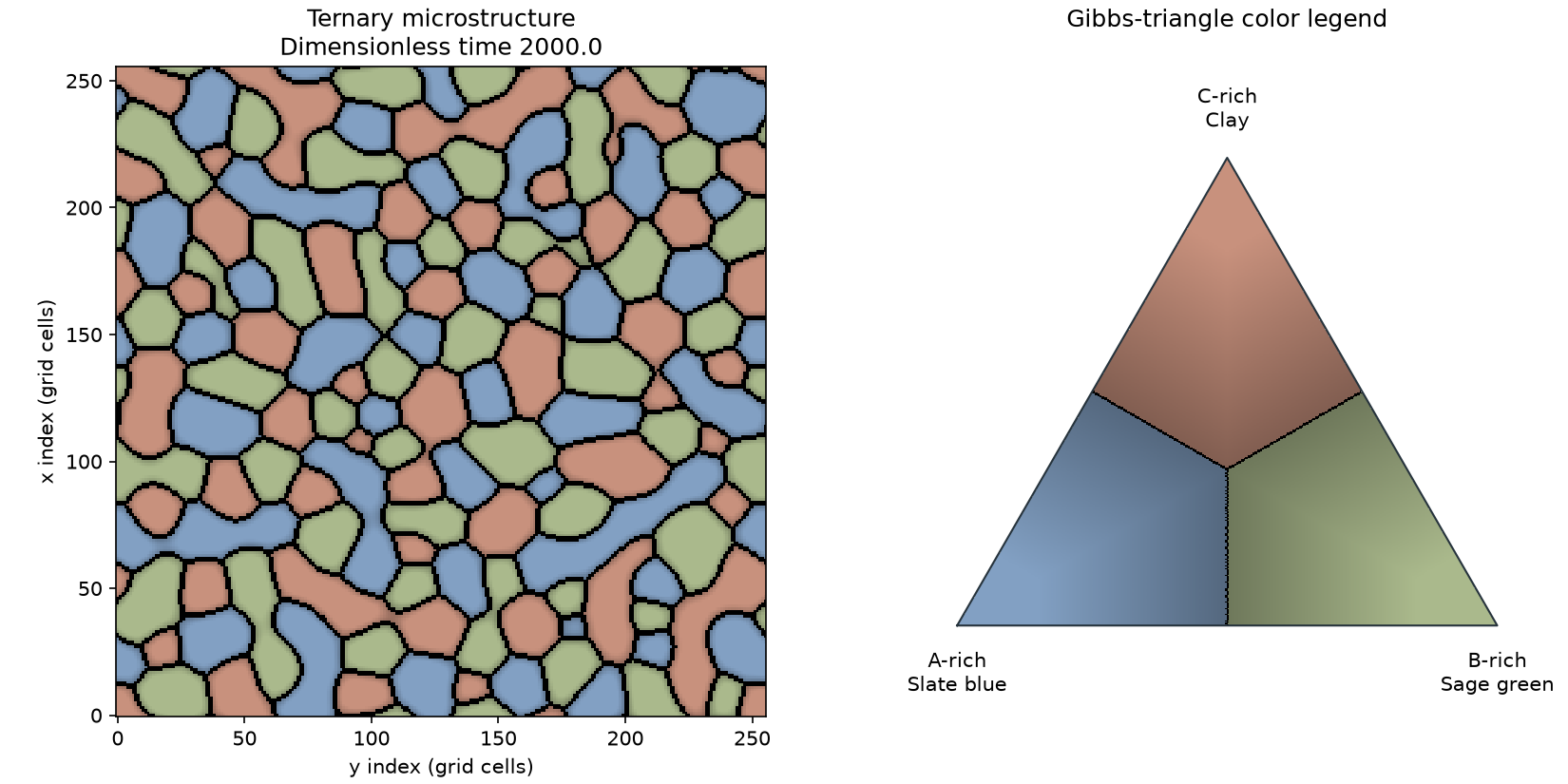

Step 9: Save the fields for structure and correlation analysis

I save the unmodified compositions and the run settings in a NumPy archive. The structure-function lesson can read any one of these fields, remove its measured mean, and calculate its spectrum and pair correlation. Spatial correlation measures a length and direction of composition variation; it does not by itself prove connectivity. I keep that question separate from Hoshen–Kopelman labeling.

Python

np.savez_compressed("ternary-fields.npz", cA=cA, cB=cB, cC=cC,
                    dx=dx, dy=dy, dt=dt, steps=steps, seed=seed)
with np.load("ternary-fields.npz") as saved:
    assert np.array_equal(saved["cA"], cA)
    deviation = saved["cA"] - saved["cA"].mean()
    structure = np.abs(np.fft.fft2(deviation))**2 / deviation.size
    covariance = np.fft.ifft2(structure).real
    assert abs(covariance[0, 0] - np.mean(deviation**2)) < 1e-12
print("Saved ternary-fields.npz; covariance normalization check passed.")