Two ways to solve inhomogeneous elasticity.
A precipitate wants to change shape. Its surroundings resist. Follow two numerical routes to the same mechanical equilibrium, with the equations and the iteration visible.
These teaching examples explain two methods used to solve mechanical equilibrium in materials with different elastic stiffnesses. The direct iteration follows my earlier research solvers. The equivalent-eigenstrain example follows the method described below, including Soumya Bandyopadhyay’s work.
My classroom notebook.
The corrected teaching edition of Elastic.ipynb builds the stiffness tensor, eigenstress, acoustic tensor and elastic energy kernel \(B_{pq}(\mathbf n)\). Change the eigenstrain and elastic anisotropy separately, then compare self and cross kernels.
Download Elastic.ipynb ↓ Open in Colab ↗
What was corrected?
The original course notebook's conversion from a stiffness matrix to a fourth-order tensor had an incorrect index mapping. This edition constructs cubic elasticity directly in indices, checks shear and tensor symmetries, and handles the zero Fourier mode explicitly. It uses a full three-dimensional tensor with in-plane Fourier directions and a specified out-of-plane eigenstrain. The two solvers below use the two-dimensional sub-block with zero out-of-plane eigenstrain. The original course file is preserved.
One physical problem.
Both examples use a smooth plate in a periodic unit square. Matrix and precipitate can have different stiffnesses and anisotropies. The mean total strain \(\mathbf E\) is prescribed. Its default value, zero, means macroscopic clamping. It does not mean zero average stress. The shape is prescribed; it does not evolve during the equilibrium solve.
Physical eigenstrain is the transformation the material would undergo without constraint. Elastic strain is total strain minus eigenstrain. Both solvers report the physical energy \(\frac12\langle(\epsilon-\epsilon^0):C:(\epsilon-\epsilon^0)\rangle\).
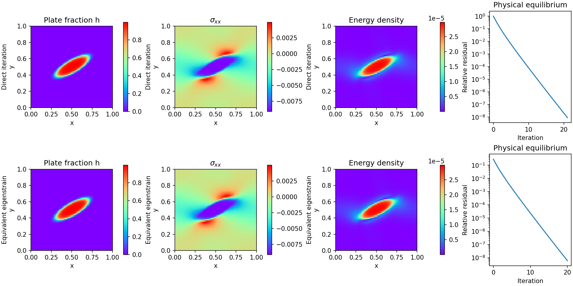
Step 1: Direct iterative perturbation.
Choose a uniform reference stiffness, split \(C=C^{ref}+\Delta C\), and put the heterogeneous contribution into a polarization stress. Recompute it after each displacement correction.
This follows the reference-stiffness approach in my earlier C and Fortran solvers and our CICP paper. Each iteration is a homogeneous Fourier solve; repeated corrections recover the heterogeneous problem. The full wavevector acoustic tensor includes the required wave-number scaling.
Step 2: Equivalent eigenstrain.
I use a uniform reference solid and find the auxiliary eigenstrain that gives it the same stress as the heterogeneous solid.
Equilibrate the reference solid, compare its stress with the physical stress, then correct \(\eta\). The notebook plots the physical eigenstrain, the equivalent eigenstrain and their difference. This makes the role of the auxiliary field visible.
The example is inspired by Soumya Bandyopadhyay's equivalent-eigenstrain work. It uses a derived constitutive-matching iteration for two solid phases. Soumya's original ferroelectric film/vacuum implementation uses an auxiliary-field relaxation law and a different geometry.
Physical insight: the auxiliary eigenstrain represents stiffness contrast mathematically. It is not a second physical transformation strain. Calculate energy using the real stiffness and physical eigenstrain.
How the inputs affect the result.
Each notebook is self-contained. Run its cells in order, edit the parameter cell, then rerun the calculation and plots. Explore soft and hard precipitates, independently chosen elastic constants, eigenstrain ratio, plate orientation and imposed mean strain. Both notebooks include an orientation sweep. The lowest sampled energy is an orientation preference for that prescribed plate, not a prediction of an evolved morphology.
Use 33 × 33 for quick exploration, then 65 × 65 and 129 × 129. Odd grids avoid Nyquist derivative ambiguity. The interface width stays fixed in physical coordinates during refinement. Numerical relaxation controls the iteration; it is not physical time.
Run the NumPy scripts
The Python scripts import routines from the other files in the same folder. The numerical routines need NumPy; plots also need Matplotlib.
python -m pip install numpy matplotlib
python direct_iteration.py
python equivalent_eigenstrain.py
python validate.py
The scripts save plots. The notebooks embed their helper routines and need no companion Python files.
Run the Julia scripts
The Julia edition follows the same equations and exposes the same helper operations. Install FFTW once, then run either solver or the cross-language validation.
julia -e 'import Pkg; Pkg.add("FFTW")'
julia DirectIteration.jl
julia EquivalentEigenstrain.jl
julia ValidateJulia.jl
Direct solver.jl ↓ · Equivalent solver.jl ↓ · Shared mathematics.jl ↓
Download Julia, NumPy, notebooks and tests ↓ Read the full derivations and instructions →
Independent checks of the solution.
The NumPy suite passes 41 numerical checks, including an exact layered-material solution, a separately assembled dense equilibrium system, Fourier displacement normalization, the homogeneous energy including its mean term, stiffness ratios from 0.2 to 5, shear loading and independent phase anisotropies. The Julia suite adds 25 cross-language checks. At five stiffness ratios it verifies equilibrium, constitutive matching, agreement between the two Julia algorithms and agreement with the NumPy reference energies. For the documented soft-plate case, changing the grid from 65 to 129 changes the energy by about 0.00125%.
The two formulations are closely related fixed-point methods, so their agreement alone is not an independent validation. Both monitor the physical equilibrium residual; the equivalent method also checks stress matching. Failed convergence raises an error. Very high contrast, voids, free outer surfaces and finite-strain mechanics are outside these examples.
Read NumPy validation results → · Read Julia validation results →
Follow the research into the code.
Direct iteration: Saswata Bhattacharyya, Tae Wook Heo, Kunok Chang and Long-Qing Chen, A Spectral Iterative Method for the Computation of Effective Properties of Elastically Inhomogeneous Polycrystals, Communications in Computational Physics 11 (2012), 726–738. Related formulations appear in Tushar Jogi's thesis, §§3.1.4–3.1.6 and Appendix B.
Equivalent eigenstrain: Soumya Bandyopadhyay's group implementation provides the motivation for the second route. These small teaching implementations expose the core equations; they are not verbatim ports of the larger research codes. New source is GPL-3.0-or-later.
Return to the interactive Elastic Stress Effects Laboratory → · Read the appendix-based kernel derivation →