Random walks and diffusion.

I begin with molecules at the origin on an unbounded two-dimensional lattice. Each step moves one lattice spacing in a cardinal direction. Position is measured in lattice spacings and time in sweeps. One sweep moves every molecule once. Mean-square displacement is the average squared distance from the starting point, in squared lattice spacings. The diffusion coefficient for this convention is 1/4 lattice-spacing squared per sweep.

Python notebook ↓ · Julia notebook ↓ · Complete collection ↓

Run notebook cells in order. Extract the complete collection without changing its folder structure: the phase-field lesson imports the original kernel from its parent folder. Use Python with NumPy, Matplotlib and Jupyter, or Julia with IJulia. Julia Fourier examples also require FFTW. The download includes installation commands and the actual check report.

Step 1: Set the positions and allowed moves

I first check the move lengths. No boundary rule is applied to the positions: the histogram window used by the complete program is only a display window.

Python

import numpy as np
rng = np.random.default_rng(7)
number = 50000
positions = np.zeros((number, 2), dtype=int)
moves = np.array([[1, 0], [-1, 0], [0, 1], [0, -1]])
assert np.all(np.sum(moves**2, axis=1) == 1)
assert np.all(positions == 0)
print("Molecules:", number)

using Random, Statistics
rng = MersenneTwister(7)
number = 50000
positions = zeros(Int, number, 2)
moves = [1 0; -1 0; 0 1; 0 -1]
@assert all(sum(moves.^2; dims=2) .== 1)
@assert all(positions .== 0)
println("Molecules: ", number)

Step 2: Take one sweep

I choose a direction independently for each molecule. After the first sweep every molecule is exactly one lattice spacing from the origin.

Python

choices = rng.integers(0, 4, number)
positions += moves[choices]
assert np.all(np.sum(positions**2, axis=1) == 1)
print("Mean-square displacement after one sweep:", np.mean(np.sum(positions**2, axis=1)))

for molecule in axes(positions, 1)
    choice = rand(rng, 1:4)
    positions[molecule, :] .+= moves[choice, :]
end
@assert all(sum(positions.^2; dims=2) .== 1)
println("First-sweep mean-square displacement: ", mean(sum(positions.^2; dims=2)))

Step 3: Measure displacement over many sweeps

The predicted ensemble mean-square displacement equals the sweep count. An individual finite sample fluctuates. I therefore use a stated statistical tolerance instead of requiring exact equality. The seed makes this NumPy run repeatable; Julia uses a different random generator.

Python

sweep_count = 100
history = [0.0, 1.0]
for sweep in range(2, sweep_count + 1):
    choices = rng.integers(0, 4, number)
    positions += moves[choices]
    history.append(float(np.mean(np.sum(positions**2, axis=1))))
relative_error = abs(history[-1] / sweep_count - 1)
assert relative_error < 0.06
print("Measured:", history[-1], "prediction:", sweep_count)
print("Relative error:", relative_error)

sweep_count = 100
history = [0.0, 1.0]
for sweep in 2:sweep_count
    for molecule in axes(positions, 1)
        choice = rand(rng, 1:4)
        positions[molecule, :] .+= moves[choice, :]
    end
    push!(history, mean(sum(positions.^2; dims=2)))
end
relative_error = abs(history[end] / sweep_count - 1)
@assert relative_error < 0.06
println("Measured: ", history[end], "; prediction: ", sweep_count)

Step 4: Individual motion and spreading

A molecule continues making discrete random steps. Diffusion describes the distribution of many molecules. The mean displacement should be small compared with the root-mean-square distance. The check below is an ensemble check for this seeded example, not a universal bound.

Python

mean_position = positions.mean(axis=0)
root_mean_square_distance = np.sqrt(history[-1])
assert np.linalg.norm(mean_position) < 0.1 * root_mean_square_distance
print("Mean position:", mean_position)
print("Root-mean-square distance:", root_mean_square_distance)

import matplotlib.pyplot as plt
fig, ax = plt.subplots()
ax.plot(range(sweep_count + 1), history, label="Measured")
ax.plot(range(sweep_count + 1), range(sweep_count + 1), "--", label="Prediction")
ax.set_xlabel("Time (sweeps)")
ax.set_ylabel("Mean-square displacement (lattice spacing squared)")
ax.legend()
plt.show()

mean_position = vec(mean(positions; dims=1))
root_mean_square_distance = sqrt(history[end])
@assert sqrt(sum(mean_position.^2)) < 0.1 * root_mean_square_distance
println("Mean position: ", mean_position)
println("Root-mean-square distance: ", root_mean_square_distance)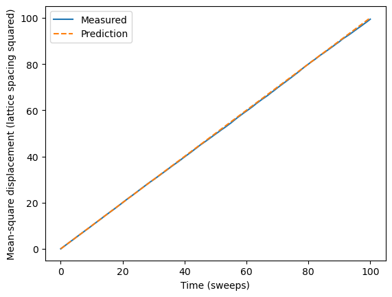

What I checked

I executed all Python notebook cells in a clean kernel and all Julia script stages. The checks apply to the short examples shown here. They do not establish grid convergence or reproduce every long simulation. Julia notebook-kernel execution is not included in these checks; the notebook code cells are identical to the tested Julia script.

Return to the code collection →