Chemical and elastic phase separation.

I use the website’s dimensionless two-dimensional model, with periodic boundaries, unit mobility and unit gradient coefficient. Composition c is a conserved field. The bulk free-energy density is c²(1-c)². Its derivative contributes 2c(1-c)(1-2c) to chemical potential. The elastic coefficient B(k) is zero for the chemical example. The elastic example uses a homogeneous 2D constitutive model with zero mean stress; it is not a calibrated alloy or a plane-strain reduction of a 3D eigenstrain.

Python notebook ↓ · Julia notebook ↓ · Complete collection ↓

Run notebook cells in order. Extract the complete collection without changing its folder structure: the phase-field lesson imports the original kernel from its parent folder. Use Python with NumPy, Matplotlib and Jupyter, or Julia with IJulia. Julia Fourier examples also require FFTW. The download includes installation commands and the actual check report.

Step 1: Create wave numbers and the initial field

I start with the chemical case. The grid spacing is one dimensionless length unit. I remove the mean of the deterministic perturbation so that the initial mean composition is exactly 0.5 to floating-point accuracy.

Python

import numpy as np
n = 64
dt = 0.2
k = 2 * np.pi * np.fft.fftfreq(n)
kx, ky = np.meshgrid(k, k, indexing="ij")
k2 = kx**2 + ky**2
row, column = np.meshgrid(np.arange(n), np.arange(n), indexing="ij")
noise = np.sin((row + 1) * 12.9898 + (column + 1) * 78.233) * 43758.5453
noise = 0.02 * (noise - np.floor(noise) - 0.5)
noise -= noise.mean()
initial = 0.5 + noise
assert abs(initial.mean() - 0.5) < 1e-12
assert k2[0, 0] == 0
print("Initial mean:", initial.mean())

using FFTW, Statistics
n = 64
dt = 0.2
k = 2π .* fftfreq(n)
kx = repeat(reshape(k, n, 1), 1, n)
ky = permutedims(kx)
k2 = kx.^2 .+ ky.^2
noise = [sin(row*12.9898 + column*78.233)*43758.5453 for row in 1:n, column in 1:n]
noise = 0.02 .* (noise .- floor.(noise) .- 0.5)
noise .-= mean(noise)
initial = 0.5 .+ noise
@assert abs(mean(initial) - 0.5) < 1e-12
@assert k2[1, 1] == 0
println("Initial mean: ", mean(initial))

Step 2: One update and my conservation check

The gradient and elastic terms are implicit; the nonlinear bulk derivative is explicit. The zero Fourier mode is unchanged because k² is zero there. I check the mean and finite values after one update. These checks do not prove energy stability.

Python

chemical_kernel = np.zeros_like(k2)
bulk_derivative = 2 * initial * (1 - initial) * (1 - 2 * initial)
numerator = np.fft.fft2(initial) - dt * k2 * np.fft.fft2(bulk_derivative)
denominator = 1 + dt * k2 * (k2 + chemical_kernel)
one_step = np.fft.ifft2(numerator / denominator).real
assert np.isfinite(one_step).all()
assert abs(one_step.mean() - initial.mean()) < 1e-12
print("Mean change after one update:", one_step.mean() - initial.mean())

chemical_kernel = zeros(size(k2))
bulk_derivative = 2 .* initial .* (1 .- initial) .* (1 .- 2 .* initial)
numerator = fft(initial) .- dt .* k2 .* fft(bulk_derivative)
denominator = 1 .+ dt .* k2 .* (k2 .+ chemical_kernel)
one_step = real.(ifft(numerator ./ denominator))
@assert all(isfinite, one_step)
@assert abs(mean(one_step) - mean(initial)) < 1e-12
println("Mean change: ", mean(one_step) - mean(initial))

Step 3: Add the elastic kernel separately

I use the existing tested kernel rather than introducing a different formula in this notebook. C11, C12 and C44 are dimensionless elastic stiffnesses here. The dilatational eigenstrain is dimensionless. I check the isotropic limit, in which the nonzero-mode kernel has no angular dependence. I also check that zero misfit removes the elastic contribution. I symmetrize conjugate Fourier partners for a real field on an even grid.

Python

def kernel(kx, ky, c11=4.0, c12=2.0, c44=3.0, eigenstrain=0.2):
    """B = E:C:E - (sigma0.n).Q^-1.(sigma0.n), E=eigenstrain*I.
    Q_ik=C_ijkl*n_j*n_l; Q11=C11*nx²+C44*ny² (not C12).
    This is a 2D constitutive model, not a reduction with epsilon_zz eigenstrain.
    """
    k2 = kx * kx + ky * ky
    radius = np.sqrt(np.where(k2 == 0, 1.0, k2))
    nx, ny = (kx / radius, ky / radius)
    q11 = c11 * nx * nx + c44 * ny * ny
    q22 = c44 * nx * nx + c11 * ny * ny
    q12 = (c12 + c44) * nx * ny
    det = q11 * q22 - q12 * q12
    det = np.where(k2 == 0, 1.0, det)
    stress = (c11 + c12) * eigenstrain
    b = 2 * (c11 + c12) * eigenstrain ** 2 - stress ** 2 * (q22 * nx * nx - 2 * q12 * nx * ny + q11 * ny * ny) / det
    return np.where(k2 == 0, 0.0, b)

angles = np.linspace(0, 2 * np.pi, 33)
isotropic = kernel(np.cos(angles), np.sin(angles), c11=4, c12=2, c44=1)
assert np.ptp(isotropic) < 1e-12
assert np.allclose(kernel(kx, ky, eigenstrain=0), 0)
elastic_kernel = kernel(kx, ky, c11=4, c12=2, c44=3, eigenstrain=0.2)
partner = (-np.arange(n)) % n
elastic_kernel = 0.5 * (elastic_kernel + elastic_kernel[np.ix_(partner, partner)])
assert np.isfinite(elastic_kernel).all()
print("Isotropic angular variation:", np.ptp(isotropic))

include("../phase_field.jl")
angles = range(0, 2π; length=33)
isotropic = kernel(cos.(angles), sin.(angles); c11=4, c12=2, c44=1)
@assert maximum(isotropic) - minimum(isotropic) < 1e-12
@assert all(abs.(kernel(kx, ky; eigenstrain=0)) .< 1e-12)
elastic_kernel = kernel(kx, ky; c11=4, c12=2, c44=3, eigenstrain=0.2)
partner = mod.(-(0:n-1), n) .+ 1
elastic_kernel = 0.5 .* (elastic_kernel .+ elastic_kernel[partner, partner])
@assert all(isfinite, elastic_kernel)
println("Isotropic angular variation: ", maximum(isotropic) - minimum(isotropic))

Step 4: Compare short evolutions with the same initial field

I advance both cases from identical fields for 50 steps. This is a short execution and conservation check. The complete program supplies longer runs and free-energy records. Timestep and spatial refinement are separate questions and have not been established by this notebook.

Python

chemical = initial.copy()
elastic = initial.copy()
for step in range(50):
    chemical_bulk = 2 * chemical * (1 - chemical) * (1 - 2 * chemical)
    chemical_spectrum = np.fft.fft2(chemical) - dt * k2 * np.fft.fft2(chemical_bulk)
    chemical = np.fft.ifft2(chemical_spectrum / (1 + dt*k2*(k2 + chemical_kernel))).real
    elastic_bulk = 2 * elastic * (1 - elastic) * (1 - 2 * elastic)
    elastic_spectrum = np.fft.fft2(elastic) - dt * k2 * np.fft.fft2(elastic_bulk)
    elastic = np.fft.ifft2(elastic_spectrum / (1 + dt*k2*(k2 + elastic_kernel))).real
for result in (chemical, elastic):
    assert np.isfinite(result).all()
    assert abs(result.mean() - initial.mean()) < 1e-10
assert np.linalg.norm(chemical - elastic) > 0
print("Final time:", 50 * dt)
print("Field RMS difference:", np.sqrt(np.mean((chemical - elastic)**2)))

import matplotlib.pyplot as plt
fig, axes = plt.subplots(1, 2, figsize=(9, 4))
for ax, field, name in zip(axes, [chemical, elastic], ["Chemical", "With elasticity"]):
    image = ax.imshow(field, vmin=0, vmax=1, origin="lower")
    ax.set_title(name)
    ax.set_xlabel("y grid index")
    ax.set_ylabel("x grid index")
fig.colorbar(image, ax=axes, label="Composition c (dimensionless)")
plt.show()

chemical = copy(initial)
elastic = copy(initial)
for step in 1:50
    chemical_bulk = 2 .* chemical .* (1 .- chemical) .* (1 .- 2 .* chemical)
    chemical_spectrum = fft(chemical) .- dt .* k2 .* fft(chemical_bulk)
    chemical .= real.(ifft(chemical_spectrum ./ (1 .+ dt .* k2 .* (k2 .+ chemical_kernel))))
    elastic_bulk = 2 .* elastic .* (1 .- elastic) .* (1 .- 2 .* elastic)
    elastic_spectrum = fft(elastic) .- dt .* k2 .* fft(elastic_bulk)
    elastic .= real.(ifft(elastic_spectrum ./ (1 .+ dt .* k2 .* (k2 .+ elastic_kernel))))
end
for result in (chemical, elastic)
    @assert all(isfinite, result)
    @assert abs(mean(result) - mean(initial)) < 1e-10
end
@assert sum(abs2, chemical .- elastic) > 0
println("Final time: ", 50 * dt)
println("Field RMS difference: ", sqrt(mean((chemical .- elastic).^2)))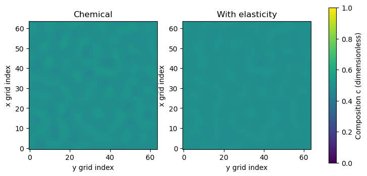

What I checked

I executed all Python notebook cells in a clean kernel and all Julia script stages. The checks apply to the short examples shown here. They do not establish grid convergence or reproduce every long simulation. Julia notebook-kernel execution is not included in these checks; the notebook code cells are identical to the tested Julia script.

Return to the code collection →