Diffusion through Fourier modes.

I calculate diffusion on a periodic line. All quantities in this example are dimensionless: position x, time t, concentration c and diffusivity D. The domain length is 2π and D = 1. Fourier wave number k identifies a spatial mode. I use exact propagation of each mode rather than an approximate time-stepping scheme.

Python notebook ↓ · Julia notebook ↓ · Complete collection ↓

Run notebook cells in order. Extract the complete collection without changing its folder structure: the phase-field lesson imports the original kernel from its parent folder. Use Python with NumPy, Matplotlib and Jupyter, or Julia with IJulia. Julia Fourier examples also require FFTW. The download includes installation commands and the actual check report.

Step 1: Define the grid

I omit the repeated endpoint of the periodic interval. I check that the grid spacing times the number of points equals the domain length.

Python

import numpy as np
n = 128
length = 2 * np.pi
spacing = length / n
x = spacing * np.arange(n)
k = 2 * np.pi * np.fft.fftfreq(n, d=spacing)
diffusivity = 1.0
assert np.isclose(n * spacing, length)
assert k[0] == 0
print("Grid points:", n, "spacing:", spacing)

using FFTW, Statistics
n = 128
length_x = 2π
spacing = length_x / n
x = spacing .* (0:n-1)
k = 2π .* fftfreq(n, 1 / spacing)
diffusivity = 1.0
@assert isapprox(n * spacing, length_x)
@assert k[1] == 0
println("Grid points: ", n, "; spacing: ", spacing)

Step 2: The initial concentration

The constant term sets the mean. Two cosine terms give two spatial wavelengths. I check the mean and transform the field back before introducing evolution.

Python

initial = 1 + 0.4 * np.cos(x) + 0.2 * np.cos(4 * x)
spectrum = np.fft.fft(initial)
assert abs(initial.mean() - 1) < 1e-12
assert np.max(np.abs(np.fft.ifft(spectrum).real - initial)) < 1e-12
print("Initial mean:", initial.mean())

initial = 1 .+ 0.4 .* cos.(x) .+ 0.2 .* cos.(4 .* x)
spectrum = fft(initial)
@assert abs(mean(initial) - 1) < 1e-12
@assert maximum(abs.(real.(ifft(spectrum)) .- initial)) < 1e-12
println("Initial mean: ", mean(initial))

Step 3: Evolve one Fourier mode

Diffusion multiplies a Fourier mode by exp(-D k² t). Higher wave numbers decay faster. I check the known concentration profile at one time; this check would catch a missing square on k.

Python

time = 0.3
decay = np.exp(-diffusivity * k**2 * time)
field = np.fft.ifft(spectrum * decay).real
exact = 1 + 0.4 * np.exp(-time) * np.cos(x) + 0.2 * np.exp(-16 * time) * np.cos(4 * x)
assert np.max(np.abs(field - exact)) < 1e-12
assert abs(field.mean() - initial.mean()) < 1e-12
print("Maximum analytical error:", np.max(np.abs(field - exact)))

time = 0.3
decay = exp.(-diffusivity .* k.^2 .* time)
field = real.(ifft(spectrum .* decay))
exact = 1 .+ 0.4 * exp(-time) .* cos.(x) .+ 0.2 * exp(-16*time) .* cos.(4 .* x)
@assert maximum(abs.(field .- exact)) < 1e-12
@assert abs(mean(field) - mean(initial)) < 1e-12
println("Maximum analytical error: ", maximum(abs.(field .- exact)))

Step 4: Repeat at several times

I keep the same initial spectrum for every time, since each evaluation gives the solution from the initial state. I check mean conservation and the decreasing concentration variation. This is not a time-step convergence study.

Python

times = [0.0, 0.02, 0.1, 0.3, 1.0]
profiles = []
variation = []
for sample_time in times:
    decay = np.exp(-diffusivity * k**2 * sample_time)
    profile = np.fft.ifft(spectrum * decay).real
    profiles.append(profile)
    variation.append(np.mean((profile - profile.mean())**2))
assert all(abs(profile.mean() - 1) < 1e-12 for profile in profiles)
assert np.all(np.diff(variation) <= 0)
print("Concentration variances:", variation)

import matplotlib.pyplot as plt
fig, ax = plt.subplots()
for sample_time, profile in zip(times, profiles):
    ax.plot(x, profile, label=f"t = {sample_time}")
ax.set_xlabel("Position x (dimensionless)")
ax.set_ylabel("Concentration c (dimensionless)")
ax.legend()
plt.show()

times = [0.0, 0.02, 0.1, 0.3, 1.0]
profiles = Vector{Float64}[]
variation = Float64[]
for sample_time in times
    sample_decay = exp.(-diffusivity .* k.^2 .* sample_time)
    profile = real.(ifft(spectrum .* sample_decay))
    push!(profiles, profile)
    push!(variation, mean((profile .- mean(profile)).^2))
end
@assert all(abs(mean(profile) - 1) < 1e-12 for profile in profiles)
@assert all(diff(variation) .<= 0)
println("Concentration variances: ", variation)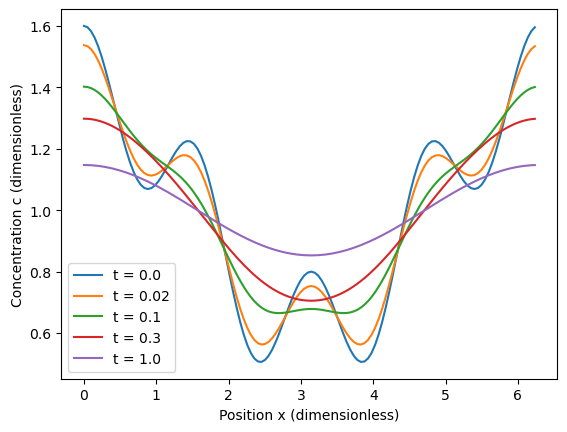

What I checked

I executed all Python notebook cells in a clean kernel and all Julia script stages. The checks apply to the short examples shown here. They do not establish grid convergence or reproduce every long simulation. Julia notebook-kernel execution is not included in these checks; the notebook code cells are identical to the tested Julia script.

Return to the code collection →