1. The model
Let c be a conserved, composition-like order parameter, with equilibrium bulk values near −1 and +1. It is dimensionless and is not directly an alloy mole fraction. We use a double-well bulk free energy and a gradient penalty on a periodic square.
In the example, M = 1, κ = 1 and the grid spacing is 1. A small random perturbation with mean zero seeds the unstable state. The continuous equation conserves mean c and dissipates free energy under periodic boundary conditions.
2. Run the example
python -m pip install numpy pillow
python spinodal_demo.py
The script writes three images, a final field array and a diagnostic CSV into spinodal_output/. It uses a 128 × 128 grid, time step 0.2, 1,600 steps and random seed 42. The images shown here were generated with that script.
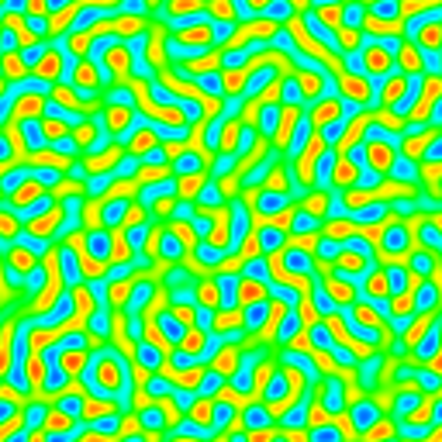
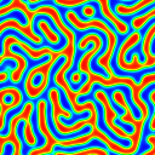
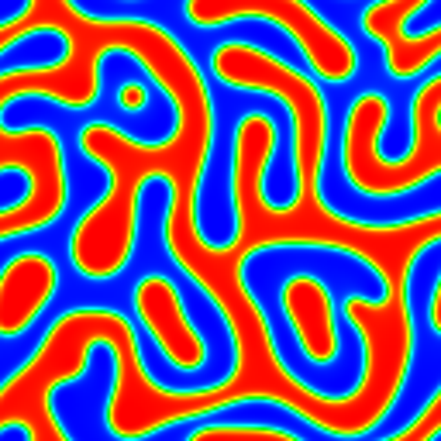
Color scale: blue = c near −1; cyan = −0.5; green = 0; yellow = 0.5; red = +1. The scale is fixed across all snapshots.
3. Understand the update
The periodic domain allows spatial derivatives to be evaluated in Fourier space. We treat the gradient penalty implicitly and the derivative of the bulk energy explicitly:
The zero wave-number mode is unchanged, which conserves the mean. The bulk term is nonlinear; evaluating it on a finite grid introduces discretization error, including aliasing. This small example does not use de-aliasing.
Do not confuse stability with accuracy.
This semi-implicit scheme is not unconditionally energy stable. If a time step produces an energy increase, refine it and inspect the trajectory. Monotone energy alone does not establish temporal or spatial convergence.
4. Check before interpreting
- Conservation: compare the initial and final mean. Drift should remain near floating-point round-off.
- Energy: plot energy density against time. The supplied diagnostic file samples every ten steps; inspect more frequently if necessary.
- Time-step sensitivity: halve Δt and double the number of steps to compare at the same final time.
- Grid convergence: refine the spacing while preserving the physical domain size. Simply increasing n with spacing fixed also enlarges the domain, so it is not a pure grid refinement.
- Initial conditions: compare statistical measures across random seeds; do not expect identical domain layouts.
5. Go further
Start with the Spinodal repository and the MicroSim documentation to connect this model with larger codes. Adding elastic energy, composition-dependent mobility or multiple components changes the physical problem and its numerical requirements.
6. Phase separation inside a particle
For the related spinodal and precipitate-growth sources, see my NRCM workshop examples. Return to Microstructures in motion for the research overview.
The example above describes phase separation throughout a periodic square. To study phase separation inside a particle, I also need to distinguish the particle from the surrounding material. A composition field describes the local mixture; a separate field can describe where the particle is.
In my embedded-particle model, \(\phi\) is a dimensionless field: \(\phi=1\) inside the particle and \(\phi=0\) outside. It changes smoothly across the particle boundary. The dimensionless function \(h(\phi)=\phi^3(10-15\phi+6\phi^2)\) changes from zero outside to one inside. I use it to combine the two bulk free-energy densities:
Here \(f_{\mathrm{bulk}}\), \(f_{\mathrm{exterior}}\) and \(f_{\mathrm{particle}}\) are free energy per unit volume before nondimensionalization; their SI units are J/m³. The supplied code uses dimensionless energies. Inside the particle, the particle free energy determines the preferred compositions. Outside, the exterior free energy determines the preferred composition. At the boundary, both terms contribute. The complete model also includes gradient energy and a composition-dependent surface term. These terms affect the interface and which phase is preferred near the particle surface.
My Julia embedded-particle code keeps the particle field fixed and evolves the composition by the Cahn–Hilliard equation with composition transport restricted by the particle field. It does not include elastic energy. Its README gives the full equations, parameters and numerical checks. The supplied short run shows a transient field; it does not establish an equilibrium core-shell or Janus morphology.
Our studies examine how phase separation and surface preference compete to produce core-shell or Janus structures: Pankaj, Bhattacharyya and Chatterjee, Acta Materialia (2022) and Modelling and Simulation in Materials Science and Engineering (2023).
Composition and structural fields have different roles
In my PRL ternary model, the auxiliary variable was the dimensionless composition \(c_A\), the fraction of component A, with \(c_A+c_B+c_C=1\). In my PCCP smoothed-boundary model, I used a separate dimensionless field \(\phi\) to impose particle boundary conditions. The choice depends on what the field represents and which physical problem is being solved.
In Sandeep’s thesis, an evolving structural field distinguishes the disordered matrix (\(\phi=0\)) from either ordered precipitate (\(\phi=1\)); composition distinguishes the two precipitates. The matrix and precipitate free energies are weighted by \(1-h(\phi)\) and \(h(\phi)\). Composition evolves through conserved transport, while the structural field evolves through an Allen–Cahn equation. This allows the precipitate boundary to move, unlike the fixed particle boundary in the Julia example. See Chapter 3, Eq. (3.77), printed p. 45, and Chapter 6, Section 6.1, printed p. 155. The model references and formulations give further details.